Tutorial: Subroto et al. (2021) - DC casting of a ternary Al alloy
This tutorial describes the steps to pre-process, run and post-process a 3D direct chill (DC) casting case that corresponds to the AA6008 conventional DC casting experiment described in Subroto et al. (2021) with directChillFoam.
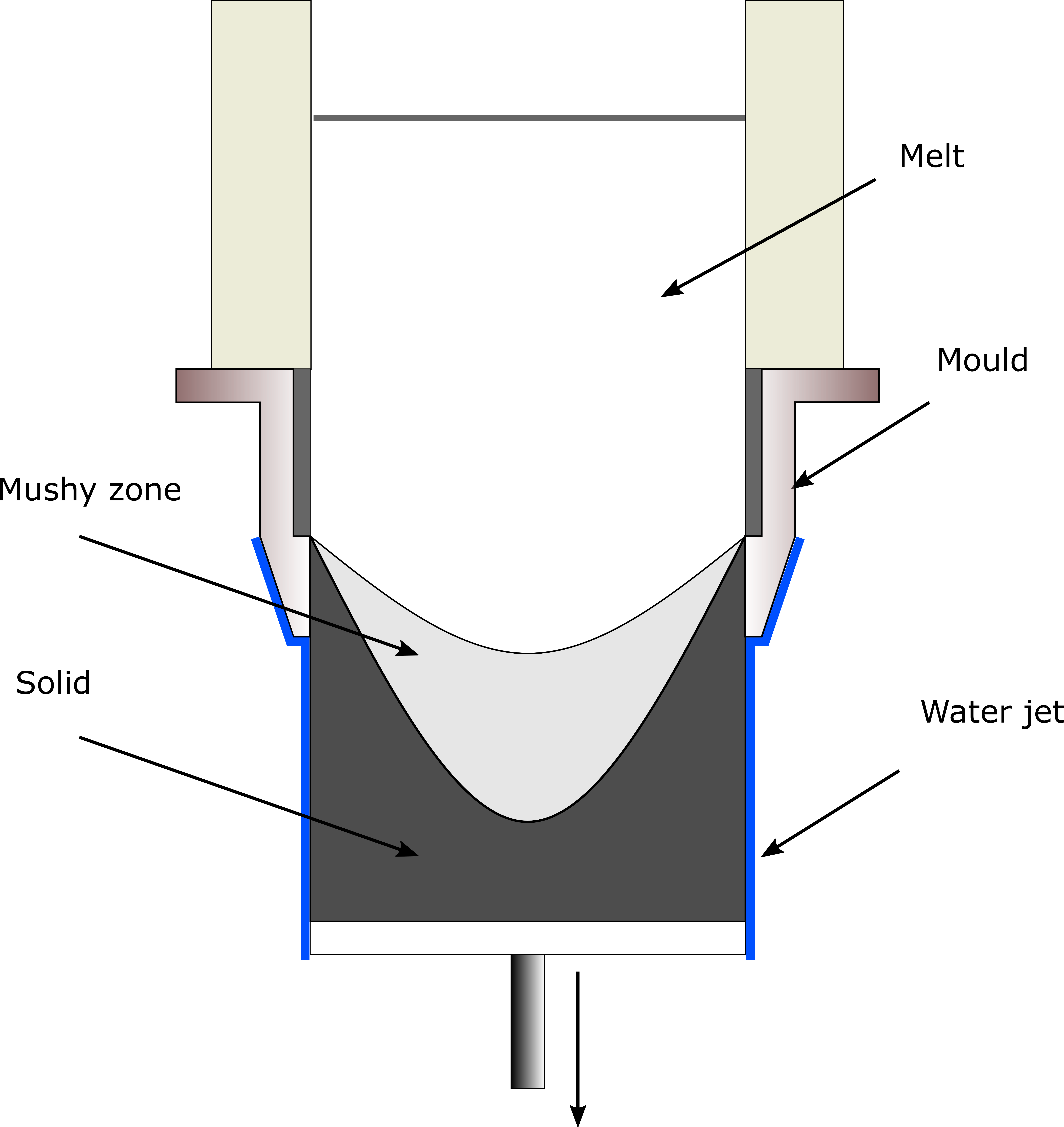
Fig. 9 The DC casting process: the melt in contact with the mould solidifies and the billet is pulled downwards by gravity as the ram is lowered. Water is sprayed at the sides of the billet providing the direct chill.
The execution time of this tutorial case is around 12 minutes when run in serial on a node with a 2.10 GHz processor.
Pre-processing
The schematic for the DC casting setup of this case is as follows:
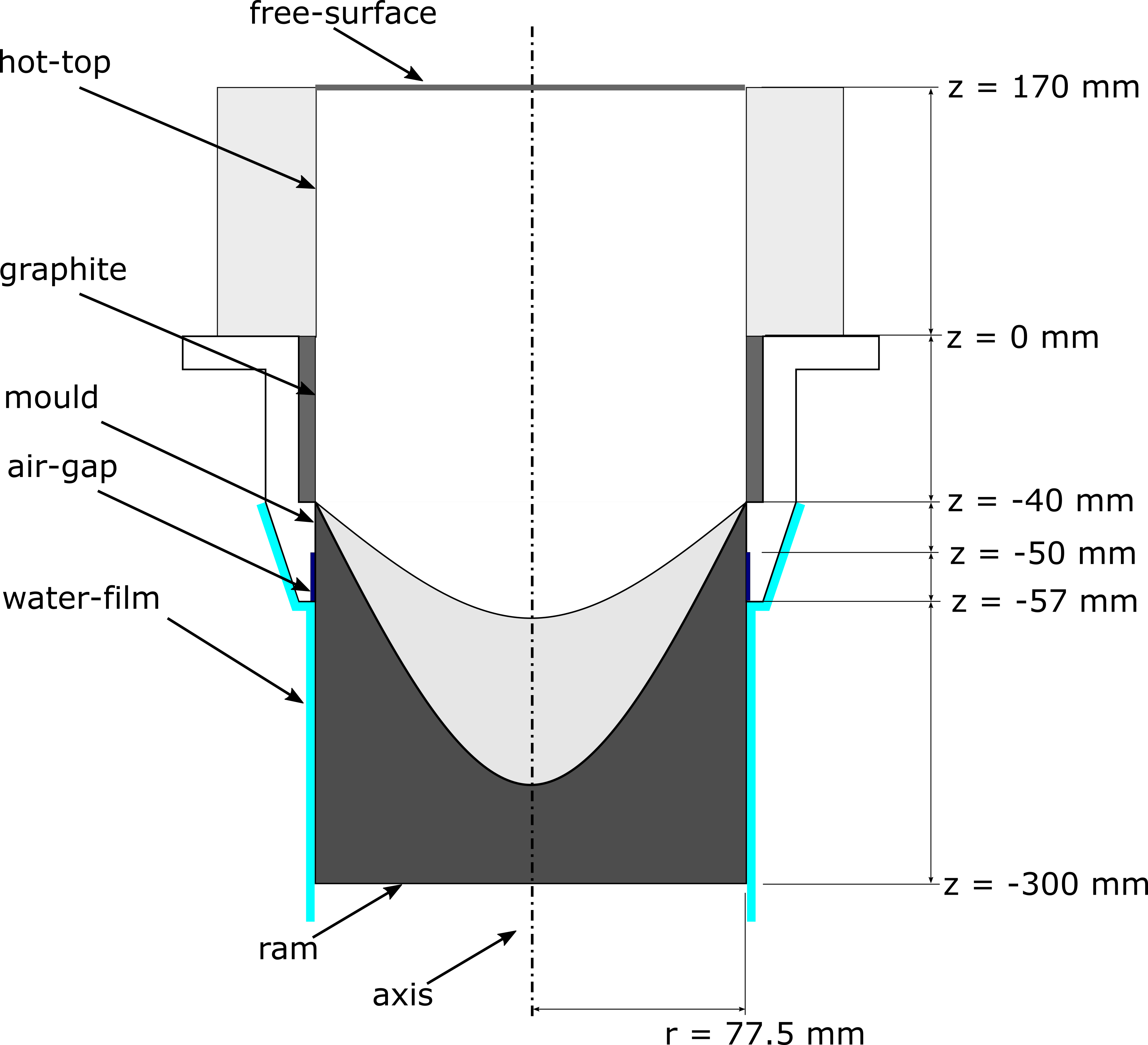
Fig. 10 Boundary patch labels and dimensions of the casting mould and billet. The image is not drawn to scale.
The first step is to generate the mesh for the case and setup the boundary conditions.
To run the pre-processing steps, change to the case directory.
$ cd directChillFoam/tutorials/heatTransfer/directChillFoam/Subroto2021
Mesh generation
The dictionary file that describes the mesh is located in the system directory.
$ cd system
Generate the blockMeshDict file using Subroto2021.system.cylinder.write_blockMeshDict() function from the system/cylinder.py script.
$ python3 cylinder.py
The axisymmetryc mesh consists of a slice of a cylinder that matches the billet dimensions. The z_points tuple list the vertices z coordinates as defined in Fig. 6. The patch names are entered in the faces list in the Lebon2020.system.cylinder.write_boundary() function.
Return to the case directory and generate the mesh using blockMesh.
$ cd ..
$ blockMesh
Boundary and initial conditions
To speed up the simulation, initialize the fields with rough estimates of temperatures (and corresponding liquid fractions) in the case directory:
$ setFields
Warning
The liquid fraction values must match the temperatures for the alloy according to the constant/tStar Foam table. Otherwise, the case can diverge.
Solute
Solute fields are dimensionless:
dimensions [0 0 0 0 0 0 0];
The fields are initialized with constant values. Use 0.6 for silicon and 0.48 for magnesium.
internalField uniform 0.6; // C.Si
internalField uniform 0.48; // C.Mg
The inlet boundary condition is a fixed value (stored in internalField):
free-surface
{
    type            fixedValue;
    value           $internalField;
}
All other boundaries are treated with a zero gradient condition.
Temperature
The mould uses the mould HTC boundary condition:
"(mould|air-gap)"
{
    type            mouldHTC;
    mode            coefficient;
    h1              uniform 1250.0;
    h2              uniform 40.0;
    Ta              constant $waterTemp;
    kappaMethod     fluidThermo;
    relaxation      1.0;
    value           uniform $waterTemp;
}
The surface of the billet that is sprayed with water jets uses the water film HTC boundary condition.
Use the Subroto2021.write_htc.write_HTC_T() function to generate the Foam temperature-htc table.
- Subroto2021.write_htc.write_HTC_T(htc_file='constant/HTC_T', func=<function rohsenhow>, T_water=372.8)
Writes the temperature-HTC foam file using the prescribed formula.
- Parameters
htc_file (str) – Relative path of HTC foam file.
func (function) – HTC function (Rohsenhow or Weckmann-Niessen).
T_water (float) – Temperature of water jet [K].
- Returns
0 if successful.
- Return type
int
water-film
{
    type            waterFilmHTC;
    mode            coefficient;
    htc
    {
        type                table;
        format              foam;
        file                "constant/HTC_Tw";
        outOfBounds         clamp;
        interpolationScheme linear;
    }
    Ta              constant $waterTemp;
    kappaMethod     fluidThermo;
    relaxation      0.3;
    value           uniform $waterTemp;
}
Velocity
The casting velocity \({U}\) is prescribed at the mould and water-cooled surface using a coded function:
"(graphite|mould|air-gap|water-film)"
{
    type            codedFixedValue;
    value           $internalField;
    redirectType    movingShell;
    name            movingShell;

    code
    #{
        // Initialize velocity with zeroes
        vectorField U(patch().size(), vector(0, 0, 0));

        // Find liquid fraction
        const scalarField& fL = this->patch().lookupPatchField<volScalarField, scalar>("melt1_alpha1");

        // Go through all face centres
        const vectorField& centre(patch().Cf());
        forAll(centre, i)
        {
            U[i].z() = -0.00233*(1-fL[i]);
        }

        // Apply the calculated velocities
         operator==(U);
    #};

    codeInclude
    #{
        // #include "fvCFD.H";
    #};
  }
The values are initialized at the casting speed in m s-1.
Solid velocity
The movingShell coded function from the liquid velocity boundary condition is reused for the solid velocity \({U_s}\) boundary prescription:
"(graphite|mould|air-gap|water-film)"
{
    type            movingShell;
    value           $internalField;
}
The values are also initialized at the casting speed in m s-1.
Physical properties
Transport properties
The transport properties are prescribed in the constant/transportProperties dictionary file. All values are in SI units. These values are available for the alloy that is being studied either in engineering tables or by calculating them using a CALPHAD software package.
Example usage:
g_env           [ 0 0 0 0 0 0 0 ] 0.7;         // Coherency fraction
rho1            [ 1 -3 0 0 0 0 0 ] 2378.65;    // Solid density
rho2            [ 1 -3 0 0 0 0 0 ] 2602.04;    // Liquid density
mu1             [ 1 -1 -1 0 0 0 0 ] 0.0010155; // Not required, but implementation requires a non-zero value
mu2             [ 1 -1 -1 0 0 0 0 ] 0.0010155; // Dynamic viscosity (of liquid)
DAS             [ 0 1 0 0 0 0 0 ] 0.000185;    // Dendrite arm spacing
Thermophysical properties
The thermophysical properties are prescribed in the constant/thermophysicalProperties dictionary file.
Solute properties
The solute properties are prescribed in the constant/soluteProperties dictionary file.
Example usage:
solutes
(
    Si
    {
        D_l   3e-9;     // Liquid mass diffusion coefficient
        kp    0.102068; // Partition coefficient
        C0    0.6;      // Initial solute concentration
        Ceut  0.32;     // Eutectic concentration
        beta  -3.7e-4;  // Solute expansion coefficient
    }

    Mg
    {
        D_l   3e-9;
        kp    0.316119;
        C0    0.48;
        Ceut  0.32;
        beta  1.3e-4;
    }
);
Note
These values are also obtained from engineering tables or by calculating them using a CALPHAD software package.
Solidification properties
The solidification properties are prescribed in the constant/fvModels dictionary file.
Example usage:
melt1
{
    type            mushyZoneSource;
    active          yes;

    mushyZoneSourceCoeffs
    {
        selectionMode   all;

        Tliq            928.236;         // Liquidus temperature [K]
        Tsol            805.503;         // Solidus temperature [K]
        L               351540.0;        // Latent heat of fusion [J/kg]
        g_env           0.7;             // Coherency fraction
        relax           0.1;             // Under-relaxation factor [0-1] - keep this value low if simulation is unstable
        castingVelocity (0 0 -0.00233);  // Casting velocity [m/s]

        tStar
        // liquid fraction-temperature table
        {
            type                table;
            format              foam;
            file                "constant/tStar";
            outOfBounds         clamp;
            interpolationScheme linear;
        }

        thermoMode      thermo;
        rhoRef          2602.044;   // Reference (solid) density [kg/m^3]
        beta            23e-6;      // Thermal expansion coefficient [1/K]
        phi             phi;        // Name of flux field
        Cu              1.522e+07;  // Mushy region momentum sink coefficient [1/s]
        q               1e-03;      // Carman-Kozeny model coefficient
    }
}
Note
These values are also obtained from engineering tables or by calculating them using a CALPHAD software package.
The tStar table can be obtained using a CALPHAD calculation using an appropriate diffusion model e.g. the lever rule or the Scheil equation. When using a non-linear model, use small (liquid fraction) steps of the order of 0.001 if the energy solver diverges.
Control
The solidification and other associated libraries must be included in the system/controlDict dictionary file.
libs (
    "libmyFvModels.so"
    "libmyFvConstraints.so"
    "libmythermophysicalTransportModels.so"
);
Discretization and solver settings
Discretization schemes are entered in the system/fvSchemes dictionary file. Upwinding is recommended for the solute equations.
divSchemes
{
    ...
    div(phi,C.Si)   bounded Gauss upwind;
    div(phi,C.Mg)   bounded Gauss upwind;
}
The number of energy corrector loops is prescribed in the PIMPLE entry of the system/fvSolution dictionary file.
PIMPLE
{
    ...
    nEnergyCorrectors 3;
}
Run the application
Once the case has been setup, run directChillFoam in the case directory:
$ cd directChillFoam/tutorials/heatTransfer/directChillFoam/Subroto2021
$ directChillFoam
Post-processing
Contour plots
The sump profile (Fig. 11) can be plotted from the VTK files that are saved in the
postProcessing directory using the Subroto2021.plot_sump.plot_sump() function.
- Subroto2021.plot_sump.plot_sump(image_name='sump.png', cmap='jet')
Plots sump contour.
- Parameters
image_name (str) – Filename of image, including path.
cmap (str or matplotlib.colormaps) – Color map for plotting contour.
- Returns
0 if successful.
- Return type
int
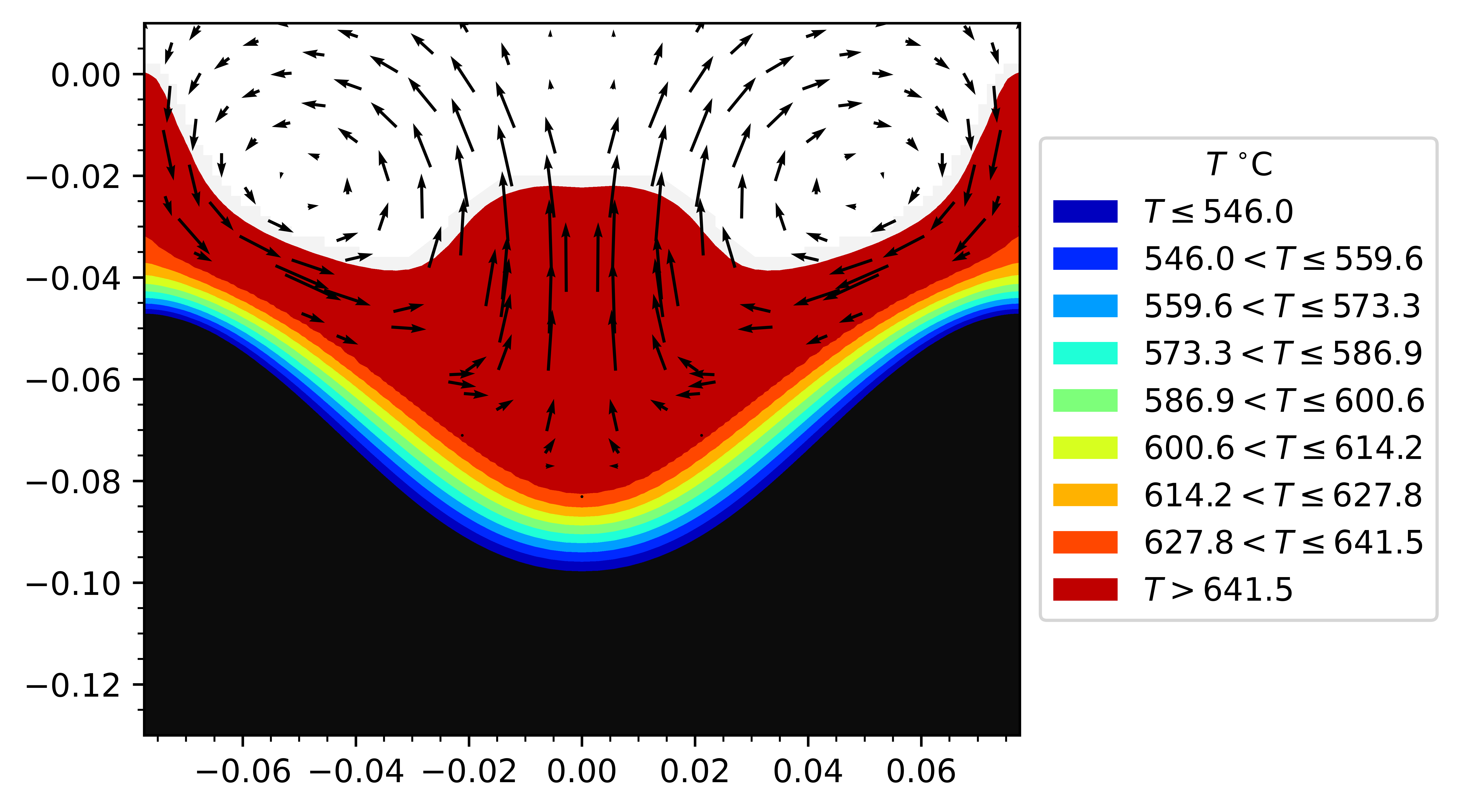
Fig. 11 Predicted sump profile.
Validation
The simulation can be verified by comparing the predicted temperatures at the
billet centre line, mid-radius and surface with experimental measurements. Use
the Subroto2021.plot_line.plot_line() function to plot Fig. 12:
- Subroto2021.plot_line.plot_line(plot_time, Experimental, Image_Path='.', offset=-0.01)
Plots temperature graphs at plot_time.
- Parameters
plot_time (str) – Time at which to plot the temperatures.
Experimental (pandas.Dataframe) – Dataframe containing experimental data.
Image_Path (str) – Absolute path of line plot.
offset (float) – Offset position of mould bottom in experiment.
- Returns
0 if successful.
- Return type
int
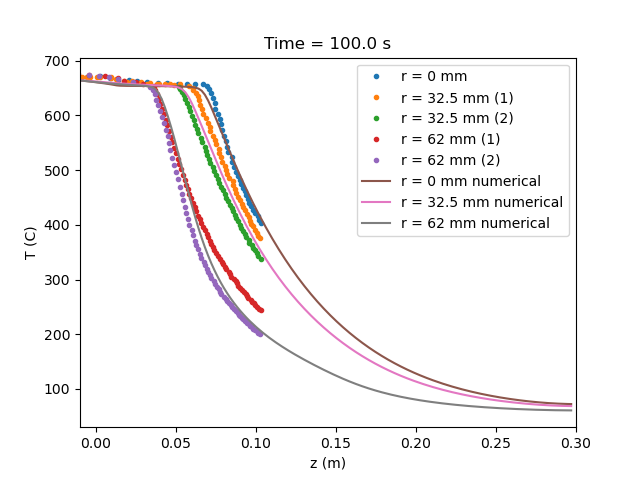
Fig. 12 Comparing the predicted temperatures (solid lines) with experimental data (markers).
